Motivation

In modern data lakehouses, where organizations manage massive and ever-growing datasets, data layout strategy plays a critical role. How data is organized, stored, and partitioned directly impacts not just query performance, but also storage efficiency, operational costs, and the system’s ability to scale.

At first glance, a non-partitioned table may seem attractive—it’s simple to create and easy to query. However, as data volumes grow, non-partitioned tables quickly become a bottleneck. Without a way to prune irrelevant data, every query risks scanning large amounts of unnecessary information, resulting in poor performance and high resource utilization.

Partitioning tables by one or more columns offers a powerful solution by physically separating data into manageable subsets. Systems can then skip over irrelevant partitions during query execution, resulting in significantly improved performance. Yet, partitioning itself introduces a new set of design challenges:

• Granularity:
  Fine-grained partitioning can lead to a flood of small files (the "small files problem" or "partition explosion"), which increases metadata overhead and slows down operations. Coarse-grained partitioning, on the other hand, can lead to data skew, where some partitions become disproportionately large, thereby hindering performance and parallelism. In some cases, such as sales data with extreme holiday spikes, there may be no ideal granularity.
  
• Number of Partition Columns:
  Using too many partition columns can also cause partition explosion, while too few can limit query optimization when filtering on non-partitioned columns.
  

In practice, designing the "perfect" partitioning scheme is often difficult, if not impossible. Real-world data is messy, dynamic, and unpredictable.

This is where clustering offers an important alternative. Rather than physically separating data into rigid partitions, clustering organizes rows based on value locality, providing many of the benefits of partitioning, such as data skipping and faster query performance, while avoiding some of its major drawbacks.

What is Clustering?

Clustering is a data layout strategy that organizes rows based on the values of one or more columns, without physically splitting the dataset into separate partitions. Instead of creating distinct directory structures, like traditional partitioning does, clustering sorts and groups related rows together within the existing storage layout.

The key idea behind clustering is locality: rows with similar values are stored close to each other. This logical organization enhances data skipping and read efficiency, enabling query engines to quickly locate and scan only the data relevant to a given query, even when no explicit partitions are present.

Unlike partitioning, which enforces strict boundaries between data segments, clustering maintains a continuous data structure while intelligently ordering rows to optimize access patterns.

How Clustering Helps

Clustering addresses several limitations of partitioning:

Enhanced Pruning for Non-Partitioned Columns

In a partitioned table, query engines can easily prune data based on partition columns, but struggle when filtering on non-partitioned fields. Clustering helps by logically grouping rows with similar values together, so even when queries filter on non-partitioned columns, irrelevant data can still be efficiently skipped.

Eliminates Partition Explosion

Partition explosion happens when too many small partitions are created, overwhelming metadata management and degrading performance. Clustering sidesteps this issue: it provides many of the data skipping benefits of partitioning without fragmenting the dataset into thousands (or millions) of physical partitions.

Better Handling of Data Skew

Real-world datasets are rarely uniform. Sales data, for instance, may experience massive volume spikes during holidays, and IoT sensor data may exhibit bursts in response to specific events. Static partitions can struggle with these uneven distributions, leading to hotspots and performance bottlenecks. Clustering, by contrast, dynamically organizes data based on value proximity, providing a more adaptive and resilient layout for skewed or unpredictable workloads.

Dremio’s Clustering Solution

Dremio’s clustering functionality is built on top of the Apache Iceberg table format, which provides the flexibility needed to manage large-scale datasets efficiently. In a clustered Iceberg table, rows within data files are physically organized so that values with similar clustering keys are stored together. Achieving this requires a method to measure and preserve data locality across multiple dimensions.

To tackle this, Dremio leverages space-filling curves—mathematical constructs such as Z-order and Hilbert curves. These curves map multidimensional data points into a one-dimensional sequence while maintaining spatial proximity as much as possible. Imagine drawing a line through a city map so that neighborhoods that are close stay close — that's what these curves do with data. In the context of clustering, this mapping enables the system to sort and organize rows in a way that maximizes data skipping during queries, without physically breaking the dataset into partitions.

Thus, clustering an Iceberg table becomes a problem of sorting rows based on their space-filling curve index values, effectively optimizing the layout to boost query performance, without the need for additional partitions.

Z-Ordering

In Dremio’s current clustering implementation, Z-ordering is used as the space-filling curve due to its speed, scalability, and strong locality preservation.

Z-order works by bitwise interleaving the binary representations of multiple columns. For example, given columns A, B, and C, Z-ordering interleaves their bits in sequence—A₁B₁C₁A₂B₂C₂...—producing a single index that captures their combined spatial relationships. This enables efficient clustering across multiple dimensions with minimal computational overhead.

Imagine you have three strands of hair — one for each column of data. Instead of laying them side by side, you braid them together, weaving one strand over the other in sequence. The braid keeps pieces from each strand close together, maintaining their relationship while combining them into a single, neat structure. Z-ordering does the same thing with data: it intertwines bits from different columns to form one organized line that preserves how close the original values were.

Why Clustering is Only Supported on Non-Partitioned Tables

At present, Dremio supports clustering only on non-partitioned tables. This design choice stems from the way clustering optimizes data layout: by ordering rows to maximize locality, clustering dramatically improves data file pruning during query execution.

For non-partitioned or under-partitioned tables, clustering offers a substantial performance boost, enabling efficient filtering without the need for rigid partition structures.

However, when a table is already partitioned, and the data within a single partition becomes excessively large, it usually signals one of two problems:

• The partitioning strategy needs refinement — possibly by increasing granularity.
  
• Data skew is occurring — where specific partitions contain a disproportionate amount of data.

In cases of severe skew, migrating the table to a clustering strategy (instead of reworking the partitions) can be a more effective and scalable solution. One of clustering’s core strengths is its ability to handle skewed and uneven data distributions gracefully, which traditional partitioning methods struggle with.

Clustering Depth and Data File Overlap

Clustering an entire dataset at once can be costly and, in many cases, unnecessary. Instead, Dremio optimizes clustering by targeting regions where data locality has degraded.

In Iceberg, data is stored in discrete data files, each covering a specific range of space-filling curve index values. If the ranges of two or more data files overlap, it signals a locality violation—meaning similar rows are scattered across multiple files rather than being grouped together. These overlapping files are candidates for rewriting and reclustering.

To quantify the effectiveness of clustering across a table, Dremio uses a metric called Clustering Depth:

• Clustering Depth measures the average number of data files that overlap at any given point across the space-filling curve index range.
  
• A lower clustering depth indicates that data is well-organized with minimal overlap, leading to faster queries.
  
• A higher clustering depth suggests that rows are poorly grouped, requiring more files to be scanned during queries.
  

By focusing clustering efforts based on overlap analysis, Dremio ensures that clustering remains incremental, efficient, and scalable, especially for vast datasets.

Clustering Depth Illustrated

To better understand how clustering depth works, let’s walk through a simple example using an orders table that has been clustered by the date column.

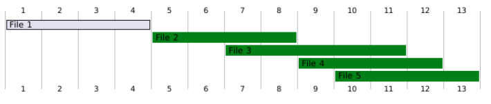
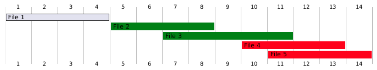
Imagine that this table is split into five data files: File1, File2, File3, File4, and File5.

Each file contains a range of dates, but because the data hasn’t been perfectly ordered yet, some files overlap (green bars), meaning they cover some of the exact dates as each other.

Here’s what happens:

• File1 does not overlap with any other file. It stands alone, covering its own unique range of dates. Therefore, its depth is 1 (just itself).
  
• File2 overlaps with File3. That means if you query for a date range that touches either File2 or File3, you might scan both. Because File2 has one overlapping neighbor (File3), its depth is 2 (itself + File3).
  
• File3 is a bit more complicated:
  
  • It overlaps with File2 (depth 2, as we just saw).
    
  • It also overlaps with Files 4 and 5. Now it has multiple overlapping neighbors!
    
  • For File3, we examine all overlaps and select the highest depth, which is 3 (including itself and the two other files).
    
• File4 overlaps with File3 and File5, so its depth is also 3.
  
• File 5 overlaps with File 3 and File 4, so its depth is 3 again.
  

Now, to summarize the overall "clutter" caused by these overlaps, we calculate the average clustering depth:

(1+2+3+3+3)/5 = 2.4

This number, 2.4, indicates, on average, how many files are intertwined across the dataset.

• A lower number (close to 1) indicates that files are well-separated, with minimal to no overlap.
  
• A higher number means that data files are more tangled, leading to more files being scanned during queries, which can slow things down.

When multiple files cover the same data ranges, queries have to scan more files to find what they need, even if most of those files contain irrelevant data.
Good clustering tries to minimize overlap, organizing the data so that a query can touch as few files as possible.

By tracking clustering depth, Dremio can measure how efficiently the data is organized — and decide whether it’s time to rewrite overlapping files to make querying faster.

Imagine stacking sheets of paper where each sheet lists dates. If too many sheets cover the same dates, you’ll have to look through a thick stack even to find a single date. Good clustering lays the sheets neatly side by side, so you can quickly pick the right one.

Calculation of Space-Filling Curve Index Range for a Data File

To organize data efficiently for clustering, we need to know where each data file sits along the space-filling curve.

In theory, the most accurate way to find a file's range would be to scan every row inside the file and compute the exact minimum and maximum indexes. However, scanning the full content of every file, especially in large tables, would be extremely expensive and impractical.

Instead, Iceberg provides a shortcut:

Each data file is already described by metadata stored in the Iceberg manifest file, which includes the minimum and maximum values for each column in the file.

We can approximate a data file’s position on the space-filling curve by:

• Treating the (min, max) values for each clustering column as the corners of a bounding box in multi-dimensional space.
  
• Then, mapping this bounding box onto a one-dimensional range along the space-filling curve.
  

By doing this, each file gets a rough index range without needing to scan the actual data inside it.

Once we have all the files mapped into index ranges, clustering becomes a simpler task:
Identify overlapping ranges, and rewrite those files to restore better locality.

Incremental Clustering Process

Clustering an entire large table all at once would be risky.

• It could take an extremely long time.
  
• It could require enormous amounts of memory, risking Out Of Memory (OOM) errors and destabilizing the system.

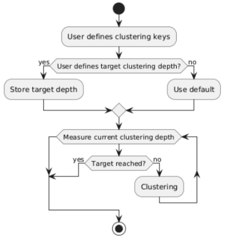
To avoid this, Dremio’s clustering process is designed to work incrementally:

Instead of rewriting everything in a single shot, clustering runs in small steps, improving the data layout gradually over time.

Each iteration of clustering:

• Targets a manageable set of files.
  
• Rewrites only the files that show the most overlap.
  
• Checks if the clustering goal (such as a target clustering depth) has been met.
  

This approach ensures that even very large datasets can be reclustered efficiently without overloading compute resources.

Users can tune how aggressive or cautious clustering is by adjusting a few important parameters:

• Maximum number of data files per iteration
  
• Maximum total size of files processed per iteration
  
• Target cluster size (which controls how big the output data files should be after clustering)
  

By fine-tuning these settings, users can balance speed, resource usage, and clustering quality based on their workload needs.

Clustering Job Illustrations

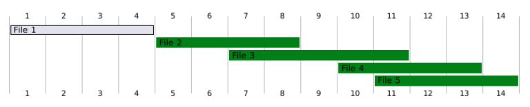
Let’s revisit the earlier example of the orders table.
We have five data files: File1, File2, File3, File4, and File5.

Before clustering:

• File2, File3, File4, and File5 overlap with each other, creating a tangled region of data.
  
• File1 does not overlap with any others and remains unaffected.
  

Now, let’s walk through what happens when Dremio performs a clustering job to resolve these overlaps.

Depending on the size and relationships between the overlapping files, three outcomes are possible:

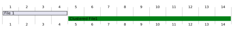
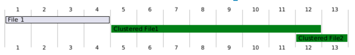
Case 1: Merge All Files into a Single Clustered File (One Iteration)

• All overlapping files (File2, File3, File4, and File5) are merged into one clustered file: ClusteredFile1.
  
• This is possible because the total size of the combined files stays below the target cluster size.
  
• Only one clustering iteration is needed, and the overlapping region is fully resolved.

Case 2: Merge into Multiple Clustered Files (Still One Iteration)

• All overlapping files are treated as part of the same logical cluster.
  
• However, after merging, the data is split into multiple clustered files (e.g., ClusteredFile1 and ClusteredFile2) because the merged size exceeds the file size target.
  
• Importantly, the files still belong to the same overall cluster — they are connected, just split for practical reasons.
  
• Only one clustering iteration is needed to clean up the overlaps.

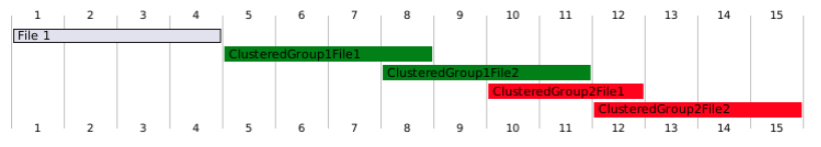
Case 3: Split into Multiple Clusters (Multiple Iterations Required)

• If the overlapping files together exceed the TARGET_CLUSTER_SIZE, Dremio first splits the files into smaller subgroups:
  
  • Subgroup1: File2 and File3
    
  • Subgroup2: File4 and File5
    
• Each subgroup is clustered separately during Iteration 1:
  
  • Subgroup1 becomes ClusteredGroup1File1 and ClusteredGroup1File2.
    
  • Subgroup2 becomes ClusteredGroup2File1 and ClusteredGroup2File2.

After the first iteration:

• ClusteredGroup1File1 and ClusteredGroup2File2 no longer overlap with anything — they are clean.
  
• However, ClusteredGroup1File2 and ClusteredGroup2File1 still overlap with each other.
  

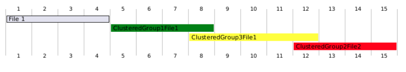
To further improve clustering and meet the target depth (e.g., depth = 1):

• Iteration 2 merges ClusteredGroup1File2 and ClusteredGroup2File1 into a new file: ClusteredGroup3File1.

At the end of Iteration 2:

• We are left with these files: File1, ClusteredGroup1File1, ClusteredGroup3File1, and ClusteredGroup2File2.
  
• These files are now properly separated, with minimal or no overlap.

Iteration 3: Final Validation

After Iteration 2 merges ClusteredGroup1File2 and ClusteredGroup2File1 into ClusteredGroup3File1,
the remaining files are:

• File1
  
• ClusteredGroup1File1
  
• ClusteredGroup3File1
  
• ClusteredGroup2File2
  

At this point:

• Each file covers a distinct range.
  
• There are no significant overlaps.
  
• The average clustering depth is now 1, meeting the clustering goal.

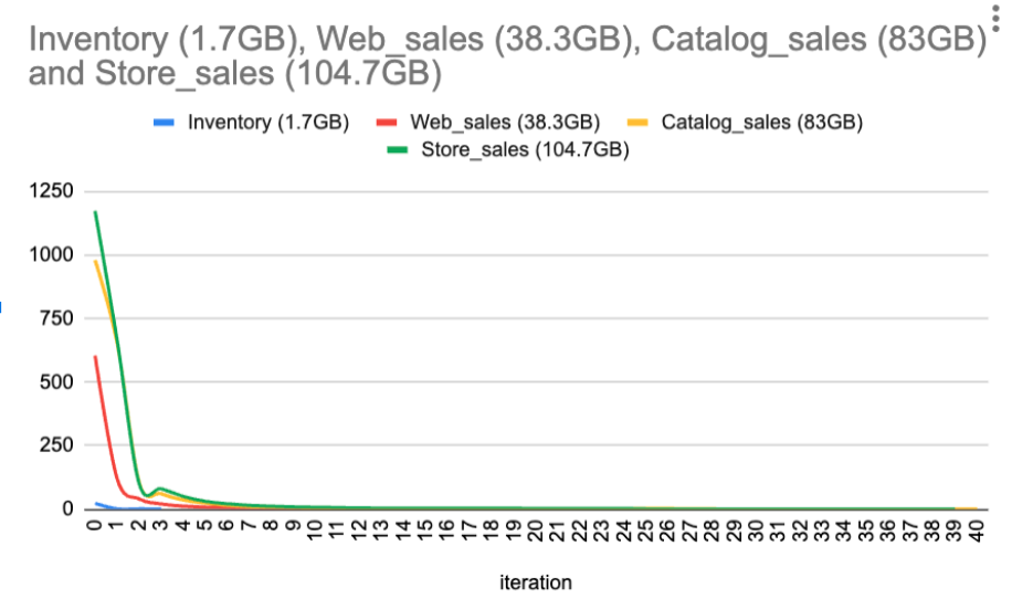
How Fast Can Clustering Converge?

Typically, considerable reductions in clustering depth occur in the early iterations. However, as the clustering depth approaches single digits, the rate of depth reduction slows down.

Tip: Users are encouraged to conduct performance experiments with different target clustering depths. In some cases, the improvements in reading performance may not be significant enough to justify further depth reduction.

Below is a diagram illustrating the clustering depth over the number of iterations using TPC-DS tables.

Advantages of Dremio’s Clustering Approach

Writing

Traditional partitioning cuts data into rigid sections based on partition columns, which can cause problems like small file proliferation and uneven data distribution.

Clustering, by contrast, organizes rows along a space-filling curve (like Z-ordering), which sorts data based on locality without creating hard boundaries.

In theory, data flows continuously along the curve.

In practice, Dremio divides the data into flexible clusters of similar size to enable parallelized writing across compute nodes.

• This process is governed by the table property dremio.clustering.target_cluster_size, which defines how large each clustered chunk should be.
  

Key benefits during writing:

• Eliminates the small files problem by grouping rows intelligently rather than rigidly partitioning them.
  
• Balances the workload across execution nodes, because clusters are sized consistently, ensuring even distribution during writes.
  
• Scales smoothly for large datasets by running clustering incrementally, which prevents overwhelming memory and compute resources.
  

This design makes Dremio’s clustering highly efficient for large-scale data processing, keeping the system stable and performant even as tables grow to massive sizes.

Reading

A key objective of any effective data layout strategy is to minimize the amount of data read during queries. The less irrelevant data the query engine touches, the faster and cheaper the query will be.

Dremio’s clustering improves read performance in two key ways:

1. Data File Level Skipping During Manifest File Scan

When clustering is based on a column like d_year, rows with similar d_year values are stored together in a small number of files.

During a query, Dremio can prune entire files based on manifest metadata before scanning any data.

For example, consider this manifest scan operation:

TableFunction(

  Table Function Type=[SPLIT_GEN_MANIFEST_SCAN], 

  ManifestFile Filter AnyColExpression=[
    (not_null(ref(name="d_year")) and ref(name="d_year") == 1999)
              ]

)

Here, the query only needs data where d_year = 1999.

Thanks to clustering, the system can quickly skip over files that don’t contain 1999, reducing the number of files it has to read.

2. Row Group Level Skipping During Data File Scan

Inside Parquet files, data is organized into row groups, each with its own (min, max) statistics for columns. When data is clustered, similar values (e.g., d_year) are stored together in the same row groups. This allows Dremio to efficiently skip entire row groups without reading them during the data scan phase.

Example data scan operation:

TableFunction(

  filters=[[Filter on `d_year`: equal(`d_year`, 1999l)]], 

  rowGroupFilters=[equal(`d_year`, 1999l)], 

  columns=[`d_date_sk`, `d_year`], 

  Table Function Type=[DATA_FILE_SCAN]

)

Here, the system applies a filter directly on the row groups, scanning only the relevant data and avoiding unnecessary I/O.

Best Practices

When to Use Clustering

Clustering shines the most in large datasets, where scanning the full data would otherwise be slow and costly.

By intelligently organizing rows based on clustering keys, clustering allows query engines to skip large portions of irrelevant data files, dramatically improving query speed and efficiency.

Best-Case Scenarios for Clustering

Clustering delivers the most significant benefit when:

• Queries commonly filter on a small set of columns.
  For example, if most queries filter on year, region, or customer_id, clustering based on these columns enables the system to prune unrelated data files and row groups quickly.
  

However, if queries filter across many different, unrelated columns (e.g., sometimes on year, other times on product_category, then city, then device_type), it becomes much harder to choose effective clustering keys.

In such cases, clustering may provide only limited performance improvement because no single key or set of keys will consistently match the query patterns.

Trade-Offs and Costs

While clustering greatly enhances performance in the right situations, it’s essential to recognize its operational costs:

• Clustering can become outdated over time, particularly in tables that are frequently updated. As new data is added or old data is modified, the initial clustering layout can deteriorate, causing the query performance gains to erode.
  
• Re-clustering is necessary to maintain performance, but even though Dremio performs clustering incrementally,
  
  • Re-clustering still consumes compute resources,
    
  • Takes time, and
    
  • Can temporarily impact query performance during background maintenance operations.
    

Thus, it’s essential to balance the benefits of clustering against the maintenance overhead, especially for datasets that experience heavy ongoing writes or updates.

Quick Summary

How to Pick Good Clustering Keys

In the current release of Dremio, users must manually select the columns used for clustering.
Choosing the right clustering keys is crucial: the better your keys align with your query patterns, the more you’ll benefit from faster reads and efficient data skipping.

Here are key recommendations for selecting effective clustering keys — some are general to all clustering approaches, and others are especially important when using Z-ordering.

Select Columns Frequently Used in Queries

Start by picking columns that appear often in query filters, such as those used in WHERE clauses.

Why?
Clustering arranges similar values close together. If your queries often filter by a particular column (e.g., order_date = 2025), clustering that column allows Dremio to prune irrelevant files and row groups quickly, making queries significantly faster.

Example:
If most queries filter on customer_id or region, those are strong candidates for clustering keys.

Include Columns Commonly Used in Joins

Columns frequently used in join conditions (e.g., ON orders.customer_id = customers.customer_id) are also excellent clustering key candidates.

Why?
When tables are clustered on join keys, Dremio can efficiently prune unnecessary data during joins, reducing both I/O and compute cost.

Example:
If a large number of queries join the Orders and Customers tables on customer_id, clustering on customer_id improves join performance.

Pay Attention to Column Cardinality

Cardinality — the number of unique values in a column — plays a major role in clustering effectiveness.

You want a balance: neither too few unique values nor too many.

• Too Low Cardinality (bad):
  If a column has only a few unique values (like a Boolean column is_active), clustering won't help much. Queries will still have to scan large sections of data because many unrelated rows are grouped.
  
• Too High Cardinality (caution):
  Columns like timestamp with nanosecond precision have millions of unique values. While this can enable very fine-grained data skipping, it can also dominate clustering, especially in Z-ordering, where bitwise interleaving favors high-cardinality columns.
  If one column overwhelms the others, overall clustering effectiveness can drop.
  

Best Practice:
Choose columns with moderate to high cardinality, but be cautious about extremely high-cardinality fields unless they are the main filter columns in your queries.

Quick Summary of Best Practices

Choosing the right clustering keys is fundamental to unlocking the full performance benefits of Dremio’s clustering capabilities. By focusing on frequently queried columns, commonly used join keys, and selecting attributes with balanced cardinality, users can dramatically improve data skipping and reduce the amount of data scanned during queries. These strategies not only speed up query execution but also optimize resource utilization, making large-scale data lakehouse environments more efficient and scalable.

However, clustering is not a "set it and forget it" solution. As datasets evolve and access patterns shift, clustering strategies may need to be revisited to maintain peak performance. By thoughtfully selecting clustering keys—and periodically reevaluating them—teams can ensure that their data remains well-organized, query performance stays high, and infrastructure costs remain under control. In a world of ever-growing data volumes, smart clustering design is no longer optional; it’s a critical component of a modern, high-performance lakehouse architecture.